Chapter 32. Bubble, Net, Stock Charts
This chapter concludes the use of Chart2 Views example by looking at how bubble, net and stock charts can be generated from spreadsheet data.
The relevant lines of chart_2_views.py are:
# Chart2View.main() ofchart_2_views.py
def main(self) -> None:
    _ = Lo.load_office(connector=Lo.ConnectPipe(), opt=Lo.Options(verbose=True))

    try:
        doc = Calc.open_doc(fnm=self._data_fnm)
        GUI.set_visible(is_visible=True, odoc=doc)
        sheet = Calc.get_sheet(doc=doc)

        chart_doc = None
        if self._chart_kind == ChartKind.AREA:
            chart_doc = self._area_chart(doc=doc, sheet=sheet)
        elif self._chart_kind == ChartKind.BAR:
            chart_doc = self._bar_chart(doc=doc, sheet=sheet)
        elif self._chart_kind == ChartKind.BUBBLE_LABELED:
            chart_doc = self._labeled_bubble_chart(doc=doc, sheet=sheet) # section 1
        elif self._chart_kind == ChartKind.COLUMN:
            chart_doc = self._col_chart(doc=doc, sheet=sheet)
        elif self._chart_kind == ChartKind.COLUMN_LINE:
            chart_doc = self._col_line_chart(doc=doc, sheet=sheet)
        elif self._chart_kind == ChartKind.COLUMN_MULTI:
            chart_doc = self._mult_col_chart(doc=doc, sheet=sheet)
        elif self._chart_kind == ChartKind.DONUT:
            chart_doc = self._donut_chart(doc=doc, sheet=sheet)
        elif self._chart_kind == ChartKind.HAPPY_STOCK:
            chart_doc = self._happy_stock_chart(doc=doc, sheet=sheet) # section 3
        elif self._chart_kind == ChartKind.LINE:
            chart_doc = self._line_chart(doc=doc, sheet=sheet)
        elif self._chart_kind == ChartKind.LINES:
            chart_doc = self._lines_chart(doc=doc, sheet=sheet)
        elif self._chart_kind == ChartKind.NET:
            chart_doc = self._net_chart(doc=doc, sheet=sheet) # section 2
        elif self._chart_kind == ChartKind.PIE:
            chart_doc = self._pie_chart(doc=doc, sheet=sheet)
        elif self._chart_kind == ChartKind.PIE_3D:
            chart_doc = self._pie_3d_chart(doc=doc, sheet=sheet)
        elif self._chart_kind == ChartKind.SCATTER:
            chart_doc = self._scatter_chart(doc=doc, sheet=sheet)
        elif self._chart_kind == ChartKind.SCATTER_LINE_ERROR:
            chart_doc = self._scatter_line_error_chart(doc=doc, sheet=sheet)
        elif self._chart_kind == ChartKind.SCATTER_LINE_LOG:
            chart_doc = self._scatter_line_log_chart(doc=doc, sheet=sheet)
        elif self._chart_kind == ChartKind.STOCK_PRICES:
            chart_doc = self._stock_prices_chart(doc=doc, sheet=sheet) # section 4

        # ...
32.1 The Bubble Chart
A bubble chart is a variation of a scatter chart where each data point shows the relationship between three variables.
Two variables are used for a bubble’s (x, y) coordinate, and the third affects the bubble’s size.
_labeled_bubble_chart() in chart_2_views.py utilizes the “World data” table in chartsData.ods (see Fig. 283).

Fig. 283 :The “World data” Table.
The data range passed to the Chart.insert_chart() uses the first three columns of the table; the Country column is added separately.
The generated scatter chart is shown in Fig. 284.

_labeled_bubble_chart() is:
# Chart2View._labeled_bubble_chart() in chart_2_views.py
def _labeled_bubble_chart(
    self, doc: XSpreadsheetDocument, sheet: XSpreadsheet
) -> XChartDocument:
    range_addr = Calc.get_address(sheet=sheet, range_name="H63:J93")
    chart_doc = Chart2.insert_chart(
        sheet=sheet,
        cells_range=range_addr,
        cell_name="A62",
        width=18,
        height=11,
        diagram_name=ChartTypes.Bubble.TEMPLATE_BUBBLE.BUBBLE,
    )
    Calc.goto_cell(cell_name="A62", doc=doc)

    Chart2.set_title(
        chart_doc=chart_doc, title=Calc.get_string(sheet=sheet, cell_name="H62")
    )
    Chart2.set_x_axis_title(
        chart_doc=chart_doc, title=Calc.get_string(sheet=sheet, cell_name="H63")
    )
    Chart2.set_y_axis_title(
        chart_doc=chart_doc, title=Calc.get_string(sheet=sheet, cell_name="I63")
    )
    Chart2.rotate_y_axis_title(chart_doc=chart_doc, angle=Angle(90))
    Chart2.view_legend(chart_doc=chart_doc, is_visible=True)

    # change the data points
    ds = Chart2.get_data_series(chart_doc)
    Props.set(
        ds[0],
        Transparency=50,
        BorderStyle=LineStyle.SOLID,
        BorderColor=CommonColor.RED,
        LabelPlacement=DataPointLabelPlacementKind.CENTER.value,
    )

    # Chart2.set_data_point_labels(
    #     chart_doc=chart_doc, label_type=DataPointLabelTypeKind.NUMBER
    # )

    # sheet_name = Calc.get_sheet_name(sheet)
    # label = f"{sheet_name}.K63"
    # names = f"{sheet_name}.K64:K93"
    # Chart2.add_cat_labels(chart_doc=chart_doc, data_label=label, data_range=names)
    return chart_doc
The transparency and border properties of all the data points are set via the DataPointProperties class for the data series. Without transparency, large bubbles could obscure or completely hide smaller bubbles.
If the call to Chart2.set_data_point_labels() is uncommented, the result is messy, as shown in Fig. 285.

Fig. 285 :Numerically Labeled Bubble Chart for the Table in Fig. 283.
Instead of labeling the bubbles with population sizes, it would be better to use the Country values (see Fig. 283).
Chart2.add_cat_labels() implements this feature, producing Fig. 286.
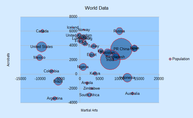
Fig. 286 :Category Labeled Bubble Chart for the Table in Fig. 283.
Chart2.add_cat_labels() employs the Country data to create an XLabeledDataSequence object which is assigned the role categories.
It is then assigned to the x-axis as category-based scale data:
# in Chart2 class
@classmethod
def add_cat_labels(
    cls, chart_doc: XChartDocument, data_label: str, data_range: str
) -> None:
    try:
        dp = chart_doc.getDataProvider()
        dl_seq = cls.create_ld_seq(
            dp=dp,
            role=DataRoleKind.CATEGORIES,
            data_label=data_label,
            data_range=data_range
        )
        axis = cls.get_axis(
            chart_doc=chart_doc, axis_val=AxisKind.X, idx=0
        )
        sd = axis.getScaleData()
        sd.Categories = dl_seq
        axis.setScaleData(sd)

        # abel the data points with these category values
        cls.set_data_point_labels(
            chart_doc=chart_doc, label_type=DataPointLabelTypeKind.CATEGORY
        )
    except ChartError:
        raise
    except Exception as e:
        raise ChartError("Error adding category lables") from e
When Chart2.set_data_point_labels() displays category data for the points, the new x-axis categories are utilized.
32.2 The Net Chart
The net chart (also called a radar chart) is useful for comparing multiple columns of data (often between three and eight columns) in a 2D arrangement that resembles a spider’s web. Although net charts have an interesting look, a lot of people dislike them (i.e. see A Critique of Radar Charts by Graham Odds).
_net_chart() in chart_2_views.py utilizes the “No of Calls per Day” table in chartsData.ods (see Fig. 287).

Fig. 287 :The “No of Calls per Day” Table.
The generated net chart is shown in Fig. 288.

_net_chart() is:
# Chart2View._net_chart() of chart_2_views.py
def _net_chart(
    self, doc: XSpreadsheetDocument, sheet: XSpreadsheet
) -> XChartDocument:
    # uses the "No of Calls per Day" table
    range_addr = Calc.get_address(sheet=sheet, range_name="A56:D63")
    chart_doc = Chart2.insert_chart(
        sheet=sheet,
        cells_range=range_addr,
        cell_name="E55",
        width=16,
        height=11,
        diagram_name=ChartTypes.Net.TEMPLATE_LINE.NET_LINE,
    )
    Calc.goto_cell(cell_name="E55", doc=doc)

    Chart2.set_title(
        chart_doc=chart_doc, title=Calc.get_string(sheet=sheet, cell_name="A55")
    )
    Chart2.view_legend(chart_doc=chart_doc, is_visible=True)
    Chart2.set_data_point_labels(
        chart_doc=chart_doc, label_type=DataPointLabelTypeKind.NONE
    )

    # reverse x-axis so days increase clockwise around net
    x_axis = Chart2.get_x_axis(chart_doc)
    sd = x_axis.getScaleData()
    sd.Orientation = AxisOrientation.REVERSE
    x_axis.setScaleData(sd)
    return chart_doc
Different net chart templates allow points to be shown, the areas filled with color, and the lines to be stacked or displayed as percentages.
_net_chart() changes the x-axis which wraps around the circumference of the chart.
By default, the axis is drawn in a counter-clockwise direction starting from the top of the net.
This order doesn’t seem right for the days of the week in this example, so the order was made clockwise, as in Fig. 288.
32.3 The Stock Chart
A stock chart is a specialized column graph for displaying stocks and shares information. All stock chart templates require at least three columns of data concerning the lowest price, highest price, and closing price of a stock (or share). It’s also possible to include two other columns that detail the stock’s opening price and transaction volume.
The stock template names reflect the data columns they utilize:
StockLowHighCloseStockOpenLowHighCloseStockVolumeLowHighCloseStockVolumeOpenLowHighClose
The names also indicate the ordering of the columns in the data range supplied to the template.
For example, StockVolumeOpenLowHighClose requires five columns of data in the order: transaction volume, opening price, lowest price, highest price, and closing price.
_happy_stock_chart() in chart_2_views.py utilizes the “Happy Systems (HASY)” table in chartsData.ods (see Fig. 289).

Fig. 289 :The “Happy Systems (HASY)” Table.
The table has six columns, the first being the x-axis categories, which are usually dates.
The other columns follow the order required by the StockVolumeOpenLowHighClose template.
The generated stock chart is shown in Fig. 290.

The chart is made up of two graphs with a common x-axis: a column graph for the stock volume on each day, and a candle-stick graph showing the lowest, opening, closing, and highest stock values.
Fig. 291 gives details of how these elements are drawn.

Fig. 291 :The Elements of a Stock Chart.
The thin red lines drawn on the columns in Fig. 291 denote the range between the lowest and highest stock value on that day. The white and black blocks represent the stock’s change between its opening and closing price. A white block (often called a “white day”) means the price has increased, while black (a “black day”) means that it has decreased.
_happy_stock_chart() is:
# Chart2View._happy_stock_chart() in chart_2_views.py
def _happy_stock_chart(
    self, doc: XSpreadsheetDocument, sheet: XSpreadsheet
) -> XChartDocument:
    # draws a fancy stock chart
    # uses the "Happy Systems (HASY)" table

    range_addr = Calc.get_address(sheet=sheet, range_name="A86:F104")
    chart_doc = Chart2.insert_chart(
        sheet=sheet,
        cells_range=range_addr,
        cell_name="A105",
        width=25,
        height=14,
        diagram_name=ChartTypes.Stock.TEMPLATE_VOLUME.STOCK_VOLUME_OPEN_LOW_HIGH_CLOSE,
    )
    Calc.goto_cell(cell_name="A105", doc=doc)

    Chart2.set_title(
        chart_doc=chart_doc, title=Calc.get_string(sheet=sheet, cell_name="A85")
    )
    Chart2.set_x_axis_title(
        chart_doc=chart_doc, title=Calc.get_string(sheet=sheet, cell_name="A86")
    )
    Chart2.set_y_axis_title(
        chart_doc=chart_doc, title=Calc.get_string(sheet=sheet, cell_name="B86")
    )
    Chart2.rotate_y_axis_title(chart_doc=chart_doc, angle=Angle(90))
    Chart2.set_y_axis2_title(chart_doc=chart_doc, title="Stock Value")
    Chart2.rotate_y_axis2_title(chart_doc=chart_doc, angle=Angle(90))

    Chart2.set_data_point_labels(
        chart_doc=chart_doc, label_type=DataPointLabelTypeKind.NONE
    )
    # Chart2.view_legend(chart_doc=chart_doc, is_visible=True)

    # change 2nd y-axis min and max; default is poor ($0 - $20)
    y_axis2 = Chart2.get_y_axis2(chart_doc)
    sd = y_axis2.getScaleData()
    # Chart2.print_scale_data("Secondary Y-Axis", sd)
    sd.Minimum = 83
    sd.Maximum = 103
    y_axis2.setScaleData(sd)

    # more stock chart code; explained in a moment...
    # ...
_happy_stock_chart() sets and rotates the secondary y-axis title, which appears on the right of the chart.
Chart2.set_y_axis2_title() and Chart2.rotate_y_axis2_title() are implemented in the same way as
set_y_axis_title() and rotate_y_axis_title() described in 29.3 Rotating Axis Titles.
_happy_stock_chart() also changes the second y-axis range; the default shows prices between $0 and $20, which is too low.
New minimum and maximum values are assigned to the axis’ scale data.
32.3.1 Modifying the Chart Dates
A common problem is that date information clutters the stock chart, making it harder to read. Fig. 290 shows that the stock template is clever enough to only draw every second date, but this is still too much information for the limited space.
One solution is to increase the x-axis interval so a tick mark (and date string) is only drawn for every third day, as in Fig. 292.

Fig. 292 :Stock Chart with Three-day Intervals for the X-Axis.
Changing the interval is implemented by adjusting the time increment for the x-axis in its ScaleData object:
# part of _happy_stock_chart() in chart_2_views.py
# ...
# change x-axis type from number to date
x_axis = Chart2.get_x_axis(chart_doc)
sd = x_axis.getScaleData()
sd.AxisType = AxisType.DATE

# set major increment to 3 days
ti = TimeInterval(Number=3, TimeUnit=TimeUnit.DAY)
tc = TimeIncrement()
tc.MajorTimeInterval = ti
sd.TimeIncrement = tc
x_axis.setScaleData(sd)
# ...
Before the interval can be changed, the axis type must be changed to be of type DATE. See ScaleData.
Another technique for making the dates easier to read is to rotate their labels.
The following code rotates each label counter-clockwise by 45 degrees:
# part of _happy_stock_chart() in chart_2_views.py
# ...
# rotate the axis labels by 45 degrees
x_axis = Chart2.get_x_axis(chart_doc)
Props.set(x_axis, TextRotation=45)
# ...
The resulting chart is shown in Fig. 293.

Fig. 293 :Stock Chart with Rotated X-Axis Labels.
Note that the template has automatically switched back to showing every date instead of every second one in Fig. 290.
32.3.2 Changing the Stock Values Appearance
This section describes two changes to the candle stick part of the chart: adjusting the colors used in the “white days” and “black days” blocks, and making the high-low stock line easier to read. The results appear in Fig. 294.

Fig. 294 :Stock Chart with Modified Candle Sticks.
A stock chart is made up of two chart types: a column chart type for the volume information, and a candle stick chart type for the stock prices.
This information can be listed by calling Chart2.print_chart_types():
Chart2.print_chart_types(chart_doc)
It produces:
No. of chart types: 2
  com.sun.star.chart2.ColumnChartType
  com.sun.star.chart2.CandleStickChartType
In order to affect the candle stick chart type’s data it is necessary to access its XChartType instance.
This can be done with the two-argument version of Chart2.find_chart_type():
# in Chart2View._happy_stock_chart() of chart_2_views.py
candle_ct = Chart2.find_chart_type(chart_doc=chart_doc, chart_type=ct)
Fig. 295 shows that the XChartType interface is supported by the ChartType service, and the CandleStickChartType subclass.

CandleStickChartType contains some useful properties, including WhiteDay and BlackDay.
These properties store sets containing multiple values from the FillProperties and LineProperties services.
They can be seen in Chart2.color_stock_bars():
# in Chart2 class
@staticmethod
def color_stock_bars(ct: XChartType, w_day_color: Color, b_day_color: Color) -> None:
    try:
        if ct.getChartType() == "com.sun.star.chart2.CandleStickChartType":
            white_day_ps = Lo.qi(XPropertySet, Props.get(ct, "WhiteDay"), True)
            Props.set(white_day_ps, FillColor=int(w_day_color))

            black_day_ps = Lo.qi(XPropertySet, Props.get(ct, "BlackDay"), True)
            Props.set(black_day_ps, FillColor=int(b_day_color))
        else:
            raise NotSupportedError(
                f'Only candel stick charts supported. "{ct.getChartType()}" not supported.'
            )
    except NotSupportedError:
        raise
    except Exception as e:
        raise ChartError("Error coloring stock bars") from e
_happy_stock_chart() calls Chart2.color_stock_bars() like so:
# in _happy_stock_chart() of chart_2_views.py
ct = ChartTypes.Stock.NAMED.CANDLE_STICK_CHART
candle_ct = Chart2.find_chart_type(chart_doc=chart_doc, chart_type=ct)
# Props.show_obj_props("Stock chart", candle_ct)
Chart2.color_stock_bars(
    ct=candle_ct,
    w_day_color=CommonColor.GREEN,
    b_day_color=CommonColor.RED
)
Making the high-low lines thicker and yellow requires access to the data series in the candle stick chart type (as shown in Fig. 295).
This is implemented by using the two- argument version of Chart2.get_data_series():
ds = Chart2.get_data_series(
    chart_doc=chart_doc,
    chart_type=ChartTypes.Stock.NAMED.CANDLE_STICK_CHART
)
The high-low lines are adjusted via the LineWidth and Color properties in the series.
The code at the end of _happy_stock_chart() is:
# end of Chart2View._happy_stock_chart() in chart_2_views.py
# ...
ct = ChartTypes.Stock.NAMED.CANDLE_STICK_CHART
# ...
# thicken the high-low line; make it yellow
ds = Chart2.get_data_series(chart_doc=chart_doc, chart_type=ct)
Lo.print(f"No. of data series in candle stick chart: {len(ds)}")
# Props.show_obj_props("Candle Stick", ds[0])
Props.set(ds[0], LineWidth=120, Color=CommonColor.YELLOW)  # LineWidth in 1/100 mm
return chart_doc
32.4 Adding a Line Graph to a Stock Chart
_stock_prices_chart() in chart_2_views.py utilizes the “Calc Guide Stock Prices” table in chartsData.ods (see Fig. 296).

Fig. 296 :The “Calc Guide Stock Prices” Table.
The stock chart is created using the first five columns, excluding the “Pork Bellies” data.
There’s no Volume column for the stocks, so the StockOpenLowHighClose template is employed.
The stock chart is shown in Fig. 297.

_stock_prices_chart() is:
# first part of Chart2View._stock_prices_chart() in chart_2_views.py
def _stock_prices_chart(self, doc: XSpreadsheetDocument, sheet: XSpreadsheet) -> XChartDocument:
    range_addr = Calc.get_address(sheet=sheet, range_name="E141:I146")
    chart_doc = Chart2.insert_chart(
        sheet=sheet,
        cells_range=range_addr,
        cell_name="E148",
        width=12,
        height=11,
        diagram_name=ChartTypes.Stock.TEMPLATE_VOLUME.STOCK_OPEN_LOW_HIGH_CLOSE,
    )
    Calc.goto_cell(cell_name="A139", doc=doc)

    Chart2.set_title(
        chart_doc=chart_doc, title=Calc.get_string(sheet=sheet, cell_name="E140")
    )
    Chart2.set_data_point_labels(
        chart_doc=chart_doc, label_type=DataPointLabelTypeKind.NONE
    )
    Chart2.set_x_axis_title(
        chart_doc=chart_doc, title=Calc.get_string(sheet=sheet, cell_name="E141")
    )
    Chart2.set_y_axis_title(chart_doc=chart_doc, title="Dollars")
    Chart2.rotate_y_axis_title(chart_doc=chart_doc, angle=Angle(90))

    # ...
A line graph showing the movement of “Pork Bellies” is added to the chart by Chart2.add_stock_line().
The additional code at the end of _stock_prices_chart() is:
# last part of Chart2View._stock_prices_chart() in chart_2_views.py
def _stock_prices_chart(self, doc: XSpreadsheetDocument, sheet: XSpreadsheet) -> XChartDocument:
    # ...
    Lo.print("Adding Pork Bellies line")
    sheet_name = Calc.get_sheet_name(sheet)
    pork_label = f"{sheet_name}.J141"
    pork_points = f"{sheet_name}.J142:J146"
    Chart2.add_stock_line(
        chart_doc=chart_doc, data_label=pork_label, data_range=pork_points
    )

    Chart2.view_legend(chart_doc=chart_doc, is_visible=True)
    return chart_doc

Chart2.view_legend(chart_doc=chart_doc, is_visible=True)
return chart_doc
The resulting change to the stock chart is shown in Fig. 298.
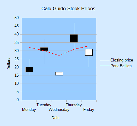
Fig. 298 :Stock Chart with Line Graph for the Table in Fig. 296.
A data series belongs to a chart type, which is part of the coordinates system. Therefore the first task is to obtain the chart’s coordinate system. A new line chart type is added to it, and an empty data series is inserted into the chart type.
The addition of a new chart type to the chart’s coordinate system is preformed by Chart2.add_chart_type().
The following adds a line chart type:
# part of Chart2.add_stock_line()
ct = cls.add_chart_type(
    chart_doc=chart_doc, chart_type=ChartTypes.Line.NAMED.LINE_CHART
)
Chart2.add_chart_type() uses Chart2.get_coord_system() to get the chart’s coordinate system, and then converts it into an XChartTypeContainer so the new chart type can be added:
#
@classmethod
def add_chart_type(
    cls, chart_doc: XChartDocument, chart_type: ChartTypeNameBase | str
) -> XChartType:
    # enusre chart_type is of correct type
    Info.is_type_enum_multi(
        alt_type="str", enum_type=ChartTypeNameBase, enum_val=chart_type, arg_name="chart_type"
    )
    try:
        ct = Lo.create_instance_mcf(
            XChartType, f"com.sun.star.chart2.{chart_type}", raise_err=True
        )
        coord_sys = cls.get_coord_system(chart_doc)
        ct_con = Lo.qi(XChartTypeContainer, coord_sys, True)
        ct_con.addChartType(ct)
        return ct
    except ChartError:
        raise
    except Exception as e:
        raise ChartError("Error adding chart type") from e
Chart2.add_chart_type() returns a reference to the new chart type, and an empty data series is added to it by converting the chart type into an XDataSeriesContainer:
# part of Chart2.add_stock_line(); see below...
ct = cls.add_chart_type(
    chart_doc=chart_doc, chart_type=ChartTypes.Line.NAMED.LINE_CHART
)
data_series_cnt = Lo.qi(XDataSeriesContainer, ct, True)

# create (empty) data series in the line chart
ds = Lo.create_instance_mcf(
    XDataSeries, "com.sun.star.chart2.DataSeries", raise_err=True
)
data_series_cnt.addDataSeries(ds)
This empty data series is filled with data points via its XDataSink interface, using the steps shown in Fig. 281.
A DataProvider service is required so that two XDataSequence objects can be instantiated, one for the label of an XLabeledDataSequence object, the other for its data.
The XDataSequence object representing the data must have its Role property set to values-y since it will become the y-coordinates of the line graph.
The task of building the XLabeledDataSequence object is handled by Chart2.create_ld_seq(), which is used in
31.5.1 Creating New Chart Data to add error bars to a scatter chart, and in 32.1 The Bubble Chart to place category labels in a bubble chart.
# part of add_stock_line() in Chart2 class
# ...
# treat series as a data sink
data_sink = Lo.qi(XDataSink, ds, True)

# build a sequence representing the y-axis data
dp = chart_doc.getDataProvider()
dl_seq = cls.create_ld_seq(
    dp=dp, role=DataRoleKind.VALUES_Y,
    data_label=data_label,
    data_range=data_range
)
# add sequence to the sink
ld_seq_arr = (dl_seq,)
data_sink.setData(ld_seq_arr)
All the preceding code fragments of this section are wrapped up inside Chart2.add_stock_line():
# in Chart2 class
@classmethod
def add_stock_line(cls, chart_doc: XChartDocument, data_label: str, data_range: str) -> None:
    try:
        # add (empty) line chart to the doc
        ct = cls.add_chart_type(
            chart_doc=chart_doc, chart_type=ChartTypes.Line.NAMED.LINE_CHART
        )
        data_series_cnt = Lo.qi(XDataSeriesContainer, ct, True)

        # create (empty) data series in the line chart
        ds = Lo.create_instance_mcf(
            XDataSeries, "com.sun.star.chart2.DataSeries", raise_err=True
        )

        Props.set(ds, Color=int(CommonColor.RED))
        data_series_cnt.addDataSeries(ds)

        # add data to series by treating it as a data sink
        data_sink = Lo.qi(XDataSink, ds, True)

        # add data as y values
        dp = chart_doc.getDataProvider()
        dl_seq = cls.create_ld_seq(
            dp=dp,
            role=DataRoleKind.VALUES_Y,
            data_label=data_label,
            data_range=data_range
        )
        ld_seq_arr = (dl_seq,)
        data_sink.setData(ld_seq_arr)
    except ChartError:
        raise
    except Exception as e:
        raise ChartError("Error adding stock line") from e
Chart2.add_stock_line() is passed a reference to the chart document, and references to the label and data for the line graph:
# part of Chart2View._stock_prices_chart() in chart_2_views.py
# ...
sheet_name = Calc.get_sheet_name(sheet)
pork_label = f"{sheet_name}.J141"
pork_points = f"{sheet_name}.J142:J146"
Chart2.add_stock_line(
    chart_doc=chart_doc,
    data_label=pork_label,
    data_range=pork_points
)
# ...