Chapter 27. Functions and Data Analysis
This chapter looks at how to utilize Calc’s spreadsheet functions directly from Python, and
then examines four of Calc’s data analysis features: pivot tables, goal seeking, and linear and nonlinear solving.
There are two nonlinear examples, one using the SCO solver, the using employing DEPS.
27.1 Calling Calc Functions from Code
Calc comes with an extensive set of functions, which are described in Appendix B of the Calc User Guide, available from https://libreoffice.org/get-help/documentation. The information is also online at https://help.libreoffice.org/Calc/Functions_by_Category, organized into eleven categories:
- Database: for extracting information from Calc tables, where the data is organized into rows.The “Database” name is a little misleading, but the documentation makes the point thatCalc database functions have nothing to do with Base databases. Chapter 13 of theCalc User Guide (“Calc as a Simple Database”) explains the distinction in detail.
Date and Time; i.e. see the
EASTERSUNDAYfunction belowFinancial: for business calculations;
Information: many of these return boolean information about cells, such as whether a cell contains text or a formula;
Logical: functions for boolean logic;
Mathematical: trigonometric, hyperbolic, logarithmic, and summation functions; e.g. see ROUND, SIN, and RADIANS below;
Array: many of these operations treat cell ranges like 2D arrays; i.e. see TRANSPOSE below;
Statistical: for statistical and probability calculations; i.e., see AVERAGE and SLOPE below;
Spreadsheet: for finding values in tables, cell ranges, and cells;
Text: string manipulation functions;
- Add-ins: a catch-all category that includes a lot of functions – extra data and time operations, conversion functions between number bases, more statistics, and complex numbers.See IMSUM and ROMAN below for examples.The “Add-ins” documentation starts at Calc Add-in Functions, and continues in
A different organization for the functions documentation is used at the OpenOffice site (Calc Functions listed by category), and is probably easy to use when browsing/searching for a suitable function.
If you know the name of the function, then a reasonably effective way of finding its documentation is to search for libreoffice calc function + the function name.
The standard way of using these functions is, of course, inside cell formulae.
But it’s also possible to call them from code via the XFunctionAccess interface.
XFunctionAccess only contains a single function, callFunction(), but it can be a bit hard to use due to data typing issues.
Calc.call_fun() creates an XFunctionAccess instance, and executes callFunction():
# in Calc class
@staticmethod
def call_fun(func_name: str, *args: any) -> object:
    args_len = len(args)
    if args_len == 0:
        arg = ()
    else:
        arg = args
    try:
        fa = Lo.create_instance_mcf(
            XFunctionAccess, "com.sun.star.sheet.FunctionAccess", raise_err=True
        )
        return fa.callFunction(func_name.upper(), arg)
    except Exception as e:
        Lo.print(f"Could not invoke function '{func_name.upper()}'")
        Lo.print(f"    {e}")
    return None
Calc.call_fun() is passed the Calc function name and and optionally an sequence of arguments.
The function’s result is returned as an Object instance.
Several examples of how to use Calc.call_fun() can be found in the Calc Funcitons example:
# in calc_functions.py
def main(self) -> None:
    with Lo.Loader(Lo.ConnectPipe()) as loader:
        doc = Calc.create_doc(loader)
        sheet = Calc.get_sheet(doc=doc, index=0)
        # round
        print("ROUND result for 1.999 is: ", end="")
        print(Calc.call_fun("ROUND", 1.999))
        # more explained below.

        Lo.close(closeable=doc, deliver_ownership=False)
The printed result is:
ROUND result for 1.999 is: 2.0
Function calls can be nested, as in:
# in calc_functions.py
print("SIN result for 30 degrees is:", end="")
print(f'{doc.call_fun("SIN", doc.call_fun("RADIANS", 30)):.3f}')
The call to RADIANS converts 30 degrees to radians.
The returned Object is accepted by the SIN function as input.
The output is: SIN result for 30 degrees is: 0.500 Many functions require more than one argument.
For instance:
# in calc_functions.py
avg = float(doc.call_fun("AVERAGE", 1, 2, 3, 4, 5))
print(f"Average of the numbers is: {avg:.1f}")
This reports the average to be 3.0.
When the Calc function documentation talks about an “array” or “matrix” argument, then the data needs to be packaged as a 2D sequence such as list or tuple. However for methods that were tested that required a matrix is showed that a list or tuple was not accepted. What does work however, is writing the 2D data into a sheet and reading it back as XCellRange values.
For example, the SLOPE function takes two arrays of x and y coordinates as input, and calculates the slope of the line through them.
So first the 2D array is written to the sheet using Calc.set_array().
Next the value are read from the sheet as XCellRange values into xrng and yrng.
Now xrng and yrng can be passed to SLOPE.
# in calc_functions.py
# the slope function only seems to work if passed XCellRange
arr = [[1.0, 2.0, 3.0], [3.0, 6.0, 9.0]]
sheet.set_array(values=arr, name="A1")
Lo.delay(500)
x_rng = sheet.get_range(range_name="A1:C1").get_cell_range()
y_rng = sheet.get_range(range_name="A2:C2").get_cell_range()
slope = float(Calc.call_fun("SLOPE", y_rng, x_rng))
print(f"SLOPE of the line: {slope}")
The slope result is 3.0, as expected.
The functions in the “Array” category almost all use 2D arrays as arguments. For example, the TRANSPOSE function is called like so:
# in calc_functions.py
arr = [[1.0, 2.0, 3.0], [4.0, 5.0, 6.0]]
sheet.set_array(values=arr, name="A1")
Lo.delay(500)
rng = sheet.get_range(range_name="A1:C3").get_cell_range()
trans_mat = doc.call_fun("TRANSPOSE", rng)
# add a little extra formatting
fl = FormatterTable(format=(".1f", ">5"))
Calc.print_array(trans_mat, fl)
The input array is in row-order, so the arr created above has two rows and three columns.
Extra formatting is use by passing Calc.print_array() a Class FormatterTable instance.
The printed transpose is:
Row x Column size: 3 x 3
  1.0  4.0
  2.0  5.0
  3.0  6.0
Note that the result of this call to Calc.call_fun() is a 2D tuple.
There are several functions for manipulating imaginary numbers, which must be written in the form of strings.
For example, IMSUM sums a series of complex numbers like so:
# in calc_functions.py
# sum two imaginary numbers: "13+4j" + "5+3j" returns 18+7j.
sum = doc.call_fun("IMSUM", "13+4j", "5+3j")
print(f"13+4j + 5+3j: {sum}")
The summed complex number is returned as the string "18+7j". This means that the Calc.call_fun() result is cast to String in this case.
Functions Help
If you can’t access the Calc documentation on functions, then calc.Calc contains two help functions: Calc.get_function_names() and Calc.print_function_info().
The former prints a very long array of function names:
List of 508 Functions
Function Names
No. of names: 508
-------------------------|--------------------------|--------------------------|--------------------------
ABS | ACCRINT | ACCRINTM | ACOS
ACOSH | ACOT | ACOTH | ADDRESS
AGGREGATE | AMORDEGRC | AMORLINC | AND
ARABIC | AREAS | ASC | ASIN
ASINH | ATAN | ATAN2 | ATANH
AVEDEV | AVERAGE | AVERAGEA | AVERAGEIF
AVERAGEIFS | B | BAHTTEXT | BASE
BESSELI | BESSELJ | BESSELK | BESSELY
BETA.DIST | BETA.INV | BETADIST | BETAINV
BIN2DEC | BIN2HEX | BIN2OCT | BINOM.DIST
BINOM.INV | BINOMDIST | BITAND | BITLSHIFT
BITOR | BITRSHIFT | BITXOR | CEILING
CEILING.MATH | CEILING.PRECISE | CEILING.XCL | CELL
CHAR | CHIDIST | CHIINV | CHISQ.DIST
CHISQ.DIST.RT | CHISQ.INV | CHISQ.INV.RT | CHISQ.TEST
CHISQDIST | CHISQINV | CHITEST | CHOOSE
CLEAN | CODE | COLOR | COLUMN
COLUMNS | COMBIN | COMBINA | COMPLEX
CONCAT | CONCATENATE | CONFIDENCE | CONFIDENCE.NORM
CONFIDENCE.T | CONVERT | CONVERT_OOO | CORREL
COS | COSH | COT | COTH
COUNT | COUNTA | COUNTBLANK | COUNTIF
COUNTIFS | COUPDAYBS | COUPDAYS | COUPDAYSNC
COUPNCD | COUPNUM | COUPPCD | COVAR
COVARIANCE.P | COVARIANCE.S | CRITBINOM | CSC
CSCH | CUMIPMT | CUMIPMT_ADD | CUMPRINC
CUMPRINC_ADD | CURRENT | DATE | DATEDIF
DATEVALUE | DAVERAGE | DAY | DAYS
DAYS360 | DAYSINMONTH | DAYSINYEAR | DB
DCOUNT | DCOUNTA | DDB | DDE
DEC2BIN | DEC2HEX | DEC2OCT | DECIMAL
DEGREES | DELTA | DEVSQ | DGET
DISC | DMAX | DMIN | DOLLAR
DOLLARDE | DOLLARFR | DPRODUCT | DSTDEV
DSTDEVP | DSUM | DURATION | DVAR
DVARP | EASTERSUNDAY | EDATE | EFFECT
EFFECT_ADD | ENCODEURL | EOMONTH | ERF
ERF.PRECISE | ERFC | ERFC.PRECISE | ERROR.TYPE
ERRORTYPE | EUROCONVERT | EVEN | EXACT
EXP | EXPON.DIST | EXPONDIST | F.DIST
F.DIST.RT | F.INV | F.INV.RT | F.TEST
FACT | FACTDOUBLE | FALSE | FDIST
FILTERXML | FIND | FINDB | FINV
FISHER | FISHERINV | FIXED | FLOOR
FLOOR.MATH | FLOOR.PRECISE | FLOOR.XCL | FORECAST
FORECAST.ETS.ADD | FORECAST.ETS.MULT | FORECAST.ETS.PI.ADD | FORECAST.ETS.PI.MULT
FORECAST.ETS.SEASONALITY | FORECAST.ETS.STAT.ADD | FORECAST.ETS.STAT.MULT | FORECAST.LINEAR
FORMULA | FOURIER | FREQUENCY | FTEST
FV | FVSCHEDULE | GAMMA | GAMMA.DIST
GAMMA.INV | GAMMADIST | GAMMAINV | GAMMALN
GAMMALN.PRECISE | GAUSS | GCD | GCD_EXCEL2003
GEOMEAN | GESTEP | GETPIVOTDATA | GROWTH
HARMEAN | HEX2BIN | HEX2DEC | HEX2OCT
HLOOKUP | HOUR | HYPERLINK | HYPGEOM.DIST
HYPGEOMDIST | IF | IFERROR | IFNA
IFS | IMABS | IMAGINARY | IMARGUMENT
IMCONJUGATE | IMCOS | IMCOSH | IMCOT
IMCSC | IMCSCH | IMDIV | IMEXP
IMLN | IMLOG10 | IMLOG2 | IMPOWER
IMPRODUCT | IMREAL | IMSEC | IMSECH
IMSIN | IMSINH | IMSQRT | IMSUB
IMSUM | IMTAN | INDEX | INDIRECT
INFO | INT | INTERCEPT | INTRATE
IPMT | IRR | ISBLANK | ISERR
ISERROR | ISEVEN | ISEVEN_ADD | ISFORMULA
ISLEAPYEAR | ISLOGICAL | ISNA | ISNONTEXT
ISNUMBER | ISO.CEILING | ISODD | ISODD_ADD
ISOWEEKNUM | ISPMT | ISREF | ISTEXT
JIS | KURT | LARGE | LCM
LCM_EXCEL2003 | LEFT | LEFTB | LEN
LENB | LINEST | LN | LOG
LOG10 | LOGEST | LOGINV | LOGNORM.DIST
LOGNORM.INV | LOGNORMDIST | LOOKUP | LOWER
MATCH | MAX | MAXA | MAXIFS
MDETERM | MDURATION | MEDIAN | MID
MIDB | MIN | MINA | MINIFS
MINUTE | MINVERSE | MIRR | MMULT
MOD | MODE | MODE.MULT | MODE.SNGL
MONTH | MONTHS | MROUND | MULTINOMIAL
MUNIT | N | NA | NEGBINOM.DIST
NEGBINOMDIST | NETWORKDAYS | NETWORKDAYS.INTL | NETWORKDAYS_EXCEL2003
NOMINAL | NOMINAL_ADD | NORM.DIST | NORM.INV
NORM.S.DIST | NORM.S.INV | NORMDIST | NORMINV
NORMSDIST | NORMSINV | NOT | NOW
NPER | NPV | NUMBERVALUE | OCT2BIN
OCT2DEC | OCT2HEX | ODD | ODDFPRICE
ODDFYIELD | ODDLPRICE | ODDLYIELD | OFFSET
OPT_BARRIER | OPT_PROB_HIT | OPT_PROB_INMONEY | OPT_TOUCH
OR | PDURATION | PEARSON | PERCENTILE
PERCENTILE.EXC | PERCENTILE.INC | PERCENTRANK | PERCENTRANK.EXC
PERCENTRANK.INC | PERMUT | PERMUTATIONA | PHI
PI | PMT | POISSON | POISSON.DIST
POWER | PPMT | PRICE | PRICEDISC
PRICEMAT | PROB | PRODUCT | PROPER
PV | QUARTILE | QUARTILE.EXC | QUARTILE.INC
QUOTIENT | RADIANS | RAND | RAND.NV
RANDBETWEEN | RANDBETWEEN.NV | RANK | RANK.AVG
RANK.EQ | RATE | RAWSUBTRACT | RECEIVED
REGEX | REPLACE | REPLACEB | REPT
RIGHT | RIGHTB | ROMAN | ROT13
ROUND | ROUNDDOWN | ROUNDSIG | ROUNDUP
ROW | ROWS | RRI | RSQ
SEARCH | SEARCHB | SEC | SECH
SECOND | SERIESSUM | SHEET | SHEETS
SIGN | SIN | SINH | SKEW
SKEWP | SLN | SLOPE | SMALL
SQRT | SQRTPI | STANDARDIZE | STDEV
STDEV.P | STDEV.S | STDEVA | STDEVP
STDEVPA | STEYX | STYLE | SUBSTITUTE
SUBTOTAL | SUM | SUMIF | SUMIFS
SUMPRODUCT | SUMSQ | SUMX2MY2 | SUMX2PY2
SUMXMY2 | SWITCH | SYD | T
T.DIST | T.DIST.2T | T.DIST.RT | T.INV
T.INV.2T | T.TEST | TAN | TANH
TBILLEQ | TBILLPRICE | TBILLYIELD | TDIST
TEXT | TEXTJOIN | TIME | TIMEVALUE
TINV | TODAY | TRANSPOSE | TREND
TRIM | TRIMMEAN | TRUE | TRUNC
TTEST | TYPE | UNICHAR | UNICODE
UPPER | VALUE | VAR | VAR.P
VAR.S | VARA | VARP | VARPA
VDB | VLOOKUP | WEBSERVICE | WEEKDAY
WEEKNUM | WEEKNUM_EXCEL2003 | WEEKNUM_OOO | WEEKS
WEEKSINYEAR | WEIBULL | WEIBULL.DIST | WORKDAY
WORKDAY.INTL | XIRR | XNPV | XOR
YEAR | YEARFRAC | YEARS | YIELD
YIELDDISC | YIELDMAT | Z.TEST | ZTEST
If you know a function name, then Calc.print_function_info() will print details about it.
For instance, information about the ROMAN function is obtained like so:
# in calc_functions.py
Calc.print_function_info("ROMAN")
The output is:
Properties for "ROMAN"":
  Id: 383
  Category: 10
  Name: ROMAN
  Description: Converts a number to a Roman numeral.
  Arguments: [Number, Mode (optional)]

No. of arguments: 2
1. Argument name: Number
  Description: 'The number to be converted to a Roman numeral must be in the 0 - 3999 range.'
  Is optional?: False

2. Argument name: Mode
  Description: 'The more this value increases, the more the Roman numeral is simplified. The value must be in the 0 - 4 range.'
  Is optional?: True
This output states that ROMAN can be called with one or two arguments, the first being a decimal,
and the second an optional argument for the amount of ‘simplification’ carried out on the Roman numeral.
For example, here are two ways to convert 999 into Roman form:
# in calc_functions.py
# Roman numbers
roman = doc.call_fun("ROMAN", 999)
# use max simplification
roman4 = doc.call_fun("ROMAN", 999, 4)
print(f"999 in Roman numerals: {roman} or {roman4}")
The output is:
999 in Roman numerals: CMXCIX or IM
Calc.get_function_names() and Calc.print_function_info() utilize the XFunctionDescriptions interface for retrieving an indexed container of function descriptions.
Each function description is an array of PropertyValue objects, which contain a Name property.
Calc.find_function() uses this organization to return a tuple of PropertyValue for a given function name:
# in Calc class (simplified, overlaods)
@staticmethod
def find_function(func_nm: str) -> Tuple[PropertyValue] | None:
    if not func_nm:
        raise ValueError("Invalid arg, please supply a function name to find.")
    try:
        func_desc = Lo.create_instance_mcf(
            XFunctionDescriptions, "com.sun.star.sheet.FunctionDescriptions", raise_err=True
        )
    except Exception as e:
        raise Exception("No function descriptions were found") from e

    for i in range(func_desc.getCount()):
        try:
            props = cast(Sequence[PropertyValue], func_desc.getByIndex(i))
            for p in props:
                if p.Name == "Name" and str(p.Value) == func_nm:
                    return tuple(props)
        except Exception:
            continue
    Lo.print(f"Function '{func_nm}' not found")
    return None
See also
The tuple of PropertyValue contains five properties: Name, Description, Id, Category, and Arguments.
The Arguments property stores an array of FunctionArgument objects which contain information about each argument’s name, description, and whether it is optional.
This information is printed by Calc.print_fun_arguments():
# in Calc class
@classmethod
def print_fun_arguments(cls, prop_vals: Sequence[PropertyValue]) -> None:
    fargs = cast(
        "Sequence[FunctionArgument]", mProps.Props.get_value(name="Arguments", props=prop_vals)
    )
    if fargs is None:
        print("No arguments found")
        return

    print(f"No. of arguments: {len(fargs)}")
    for i, fa in enumerate(fargs):
        print(f"{i+1}. Argument name: {fa.Name}")
        print(f"  Description: '{fa.Description}'")
        print(f"  Is optional?: {fa.IsOptional}")
        print()
Calc.print_function_info() calls Calc.find_function() to report on a complete function:
# in Calc class (simplified)
@classmethod
def print_function_info(cls, func_name: str) -> None:
    prop_vals = cls.find_function(func_name)
    if prop_vals is None:
        return
    Props.show_props(func_name, prop_vals)
    cls.print_fun_arguments(prop_vals)
    print()
27.2 Pivot Tables
Pivot tables are explained in detail in chapter 8 of the Calc User’s Guide.
They allow a user to view a spreadsheet consisting of columns of data in a variety of table formats, thereby highlighting the relationships between the columns.
For example, Fig. 216 shows the small spreadsheet in pivottable1.ods of the Pivot Table example.

Fig. 216 :The pivottable1.ods Spreadsheet.
The spreadsheet uses a database-like organization, with each row acting as a record, and each column is a different type/kind of information. This formatting style is described in chapter 13 “Calc as a Simple Database” in the User Guide.
The drawback of this kind of data structuring is that it can be difficult to see the underlying relationships between the columns; this is where pivot tables can help.
For example, a pivot table can be generated showing how the Category column affects Revenue (see Fig. 217).

Fig. 217 :Category Affecting Revenue
Note that the pivot table shows the revenue sum in column B, since several revenue entries in the original sheet are covered by each category.
Alternatively, it’s possible to see how Period and Category interact to affect the revenue, as in Fig. 218.

Fig. 218 :Period and Category Affect on Revenue
The ordering of the Period values can be changed by clicking on the arrow next to the Period text in cell A2, then selecting a custom sort (i.e. Jan, Feb, Mar, etc.).
The Total Result row and column are added automatically, and can be changed easily.
It’s also possible to change the way that the revenue data is grouped (i.e. it can be averaged instead of being summed).
Pivot tables are straightforward to create and modify via Calc’s GUI, starting from the Data, Pivot Table, Create menu item. Calc automatically selects all the cells used in the database-like table like the one in Fig. 216, and displays the layout dialog shown in Fig. 219.

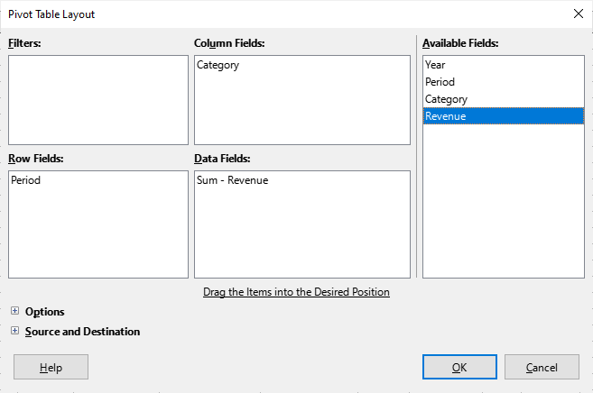
Fig. 219 :The Pivot Table Layout GUI.
The right-most “Available Fields” list contains the names of the columns in the sheet, while the other four fields (Filters, Column, Row, and Data) are empty. Fig. 219 shows a bug in the current version of the Pivot Table GUI – the addition of a “Data” name in the “Column” fields list. This name can be ignored since it doesn’t appear in the rendered pivot table.
The pivot table layout in Fig. 220 is easily created by dragging the Period name to the Row fields list,
Category to the Column fields list, and Revenue to the Data fields list, where it’s converted into Sum - Revenue.
Pivot Tables in the API
The Calc API refers to pivot tables by their old Office name, DataPilot tables. The relationships between the DataPilotservices and interfaces are shown in Fig. 221.

Fig. 221 :The DataPilot Services and Interfaces.
Fig. 221 is best understood by reading downwards: a DataPilotTables service (note the s) is a sequence of DataPilotTable services.
Each table contains a DataPilotFields service (note the s) which manages a sequence of DataPilotField objects.
Each DataPilotField is a named property set, representing a column in the source sheet.
For example, in the following code, four pilot fields will be created for the pivottable1.ods sheet shown in Fig. 216,
one each for the columns named Year, Period, Category, and Revenue.
Fig. 221 mentions one of the more important services DataPilotDescriptor, which does the hard work of converting sheet columns into pilot fields. DataPilotDescriptor is also responsible for assigning each pilot field to one of the Filters, Column, Row, or Data field lists.
The pivot_table1.py example illustrates how to create the pivot table shown in Fig. 218.
The program begins by opening the pivottable1.ods file (Fig. 216):
# in pivot_table1.py
def main(self) -> None:
    loader = Lo.load_office(Lo.ConnectSocket())

    try:
        doc = CalcDoc(Calc.open_doc(fnm=self._fnm, loader=loader))

        doc.set_visible()

        sheet = doc.get_sheet()
        dp_sheet = doc.insert_sheet(name="Pivot Table", idx=1)

        self._create_pivot_table(sheet=sheet, dp_sheet=dp_sheet)
        dp_sheet.set_active()

        if self._out_fnm:
            doc.save_doc(fnm=self._out_fnm)

        msg_result = MsgBox.msgbox(
            "Do you wish to close document?",
            "All done",
            boxtype=MessageBoxType.QUERYBOX,
            buttons=MessageBoxButtonsEnum.BUTTONS_YES_NO,
        )
        if msg_result == MessageBoxResultsEnum.YES:
            doc.close_doc()
            Lo.close_office()
        else:
            print("Keeping document open")

    except Exception:
        Lo.close_office()
        raise
A second sheet (called dp_sheet) is created to hold the generated pivot table, and _create_pivot_table() is called:
# in pivot_table1.py
def _create_pivot_table(
    self, sheet: CalcSheet, dp_sheet: CalcSheet
) -> XDataPilotTable | None:
    cell_range = sheet.find_used_range()
    print(f"The used area is: { cell_range.get_range_str()}")
    print()

    dp_tables = sheet.get_pilot_tables()
    dp_desc = dp_tables.createDataPilotDescriptor()
    dp_desc.setSourceRange(cell_range.get_address())

    # XIndexAccess fields = dpDesc.getDataPilotFields();
    fields = dp_desc.getHiddenFields()
    field_names = Lo.get_container_names(con=fields)
    print(f"Field Names ({len(field_names)}):")
    for name in field_names:
        print(f"  {name}")

    # properties defined in DataPilotField

    # set column field
    props = Lo.find_container_props(con=fields, nm="Category")
    Props.set(props, Orientation=DataPilotFieldOrientation.COLUMN)

    # set row field
    props = Lo.find_container_props(con=fields, nm="Period")
    Props.set(props, Orientation=DataPilotFieldOrientation.ROW)

    # set data field, calculating the sum
    props = Lo.find_container_props(con=fields, nm="Revenue")
    Props.set(props, Orientation=DataPilotFieldOrientation.DATA)
    Props.set(props, Function=GeneralFunction.SUM)

    # place onto sheet
    dest_addr = dp_sheet.get_cell_address(cell_name="A1")
    dp_tables.insertNewByName("PivotTableExample", dest_addr, dp_desc)
    dp_sheet.set_col_width(width=60, idx=0)
    # A column; in mm

    dp_tables2 = dp_sheet.get_pilot_tables()
    return self._refresh_table(
        dp_tables=dp_tables2, table_name="PivotTableExample"
    )
All the sheet’s data is selected by calling Calc.find_used_range().
Then Calc.get_pilot_tables() obtains the DataPilotTables service:
# in Calc class
@staticmethod
def get_pilot_table(dp_tables: XDataPilotTables, name: str) -> XDataPilotTable:
    try:
        otable = dp_tables.getByName(name)
        if otable is None:
            raise Exception(f"Did not find data pilot table '{name}'")
        result = Lo.qi(XDataPilotTable, otable, raise_err=True)
        return result
    except Exception as e:
        raise Exception(f"Pilot table lookup failed for '{name}'") from e

get_pivot_table = get_pilot_table
Calc.get_pilot_tables() utilizes the XDataPilotTablesSupplier interface of the Spreadsheet service to obtain the DataPilotTables service.
pivot_table1.py’s task is to create a new pilot table, which it does indirectly by creating a new pilot description. After this pilot description has been initialized, it will be added to the DataPilotTables service as a new pilot table.
An empty pilot description is created by calling XDataPilotTables.createDataPilotDescriptor():
# in pivot_table1.py
dp_tables = Calc.get_pilot_tables(sheet)
dp_desc = dp_tables.createDataPilotDescriptor()
The new XDataPilotDescriptor reference (dp_desc) creates a pilot table by carrying out two tasks- loading the sheet data into the pilot table,
and assigning the resulting pilot fields to the Filters, Column, Row, and Data fields in the descriptor.
This latter task is similar to what the Calc user does in the GUI’s layout window in Fig. 220.
The descriptor is assigned a source range that spans all the data:
dp_desc.setSourceRange(Calc.get_address(cell_range))
It converts each detected column into a DataPilotField service, which is a named property set; the name is the column heading.
These pilot fields are conceptually stored in the “Available Fields” list shown in the layout window in Fig. 220,
and are retrieved by calling XDataPilotDescriptor.getHiddenFields():
# in pivot_table1.py
fields = dp_desc.getHiddenFields()
It’s useful to list the names of these pilot fields:
# in pivot_table1.py
field_names = Lo.get_container_names(con=fields)
print(f"Field Names ({len(field_names)}):")
for name in field_names:
    print(f"  {name}")
The output for the spreadsheet in Fig. 216 is:
Field Names (5):
  Year
  Period
  Category
  Revenue
  Data
This list includes the strange “Data” pilot field which you may remember also cropped up in the layout window in Fig. 219.
The second task is to assign selected pilot fields to the Filters, Column, Row, and Data field lists.
The standard way of doing this is illustrated below for the case of assigning the Category pilot field to the Column field list:
# in PivotTable1._create_pivot_table()
props = Lo.find_container_props(con=fields, nm="Category")
Props.set(props, Orientation=DataPilotFieldOrientation.COLUMN)
The fields variable refers to all the pilot fields as an indexed container.
Lo.find_container_props() searches through that container looking for the specified field name.
# in Lo class
@classmethod
def find_container_props(cls, con: XIndexAccess, nm: str) -> XPropertySet | None:
    if con is None:
        raise TypeError("Container is null")
    for i in range(con.getCount()):
        try:
            el = con.getByIndex(i)
            named = cls.qi(XNamed, el)
            if named and named.getName() == nm:
                return cls.qi(XPropertySet, el)
        except Exception:
            cls.print(f"Could not access element {i}")
    cls.print(f"Could not find a '{nm}' property set in the container")
    return None
The returned property set is an instance of the DataPilotField service, so a complete list of all the properties can be found in its documentation.
The important property for our needs is Orientation which can be assigned a DataPilotFieldOrientation constant, whose values are HIDDEN, COLUMN, ROW, PAGE, and DATA,
representing the field lists in the layout window.
Once the required pilot fields have been assigned to field lists, the new pivot table is added to the other tables and to the sheet by calling XDataPilotTables.insertNewByName().
It takes three arguments: a unique name for the table, the cell address where the table will be drawn, and the completed pilot descriptor:
# in PivotTable1._create_pivot_table()
dest_addr = Calc.get_cell_address(sheet=dp_sheet, cell_name="A1")
dp_tables.insertNewByName("PivotTableExample", dest_addr, dp_desc)
This code should mark the end of the _create_pivot_table() method, but it was found that more complex pivot tables would often not be correctly drawn.
The cells in the Data field would be left containing the word #VALUE!.
This problem can be fixed by explicitly requesting a refresh of the pivot table, using:
# in PivotTable1._create_pivot_table()
def _create_pivot_table(
    self, sheet: CalcSheet, dp_sheet: CalcSheet
) -> XDataPilotTable | None:
    # ...
    dp_tables2 = dp_sheet.get_pilot_tables()
    return self._refresh_table(
        dp_tables=dp_tables2, table_name="PivotTableExample"
    )

def _refresh_table(
    self, dp_tables: XDataPilotTables, table_name: str
) -> XDataPilotTable | None:
    nms = dp_tables.getElementNames()
    print(f"No. of DP tables: {len(nms)}")
    for nm in nms:
        print(f"  {nm}")

    dp_table = Calc.get_pilot_table(dp_tables=dp_tables, name=table_name)
    if dp_table is not None:
        dp_table.refresh()
    return dp_table
Calc.get_pilot_table() searches XDataPilotTables, which is a named container of XDataPilotTable objects.
Oddly enough, it’s not enough to call Calc.get_pilot_table() on the current XDataPilotTables reference (called dp_tables in _create_pivot_table()), since the new pivot table isn’t found.
27.3 Seeking a Goal
The Tools, Goal Seek menu item in Calc allows a formula to be executed ‘backwards’. Instead of supplying the input to a formula, and obtaining the formula’s result, the result is given and “goal seek” works backwards through the formula to calculate the value that produces the result.
The Calc Goal Seek example contains several uses of “goal seeking”. It begins like so:
# in goal_seek.py
def main(self) -> None:
    with Lo.Loader(connector=Lo.ConnectPipe()) as loader:
        doc = CalcDoc(Calc.create_doc(loader))
        sheet = doc.get_sheet(0)
        gs = doc.qi(XGoalSeek, True)

        # -------------------------------------------------
        # x-variable and starting value
        cell1 = sheet.get_cell(cell_name="C1")
        # formula
        cell2 = cell1.get_cell_down()
        cell2.set_val("=SQRT(C1)")
        x = cell1.goal_seek(
            gs=gs, formula_cell_name=cell2.cell_obj, result=4.0
        )
        print(f"x == {x}\n")  # 16.0

        # more goal seek examples ...
Goal seek functionality is accessed via the XGoalSeek interface of the document.
Also, a spreadsheet is needed to hold an initial guess for the input value being calculated (which I’ll call the x-variable), and for the formula.
In the example above, the x-variable is stored in cell C1 with an initial value of 9, and its formula (sqrt(x)) in cell C2.
Calc.goal_seek() is passed the cell names of the x-variable and formula, and the formula’s result, and returns the x-value that produces that result.
In the example above, Calc.goal_seek() returns 16.0, because that’s the input to sqrt() that results in 4.
Calc.goal_seek() is defined as:
# in Calc class
@classmethod
def goal_seek(
    cls, gs: XGoalSeek, sheet: XSpreadsheet, cell_name: str,
    formula_cell_name: str, result: numbers.Number
) -> float:
    xpos = cls._get_cell_address_sheet(sheet=sheet, cell_name=cell_name)
    formula_pos = cls._get_cell_address_sheet(sheet=sheet, cell_name=formula_cell_name)

    goal_result = gs.seekGoal(formula_pos, xpos, f"{float(result)}")
    if goal_result.Divergence >= 0.1:
        Lo.print(f"NO result; divergence: {goal_result.Divergence}")
        raise GoalDivergenceError(goal_result.Divergence)
    return goal_result.Result
The heart of Calc.goal_seek() is a call to XGoalSeek.seekGoal() which requires three arguments:
the address of the x-variable cell, the address of the formula cell, and a string representing the formula’s result.
The call returns a GoalResult object that contains two fields:
Result holds the calculated x-value, and Divergence measures the accuracy of the x-value.
If the goal seek has succeeded, then the Divergence value should be very close to 0; if it failed to find an x-value then Divergence may be very large since it measures the amount the x-value
changed in the last iteration of the “goal seek” algorithm.
Not sure what algorithm “goal seek” employs, but it’s most likely a root-finding methods, such as Newton-Raphson or the secant method.
These may fail for a poor choice of starting x-value or if the formula function has a strange derivative (an odd curvature).
This can be demonstrated by asking “goal seek” to look for an impossible x-value, such as the input that makes sqrt(x) == -4:
# in goal_seek.py
try:
    x = cell1.goal_seek(gs=gs, formula_cell_name=cell2.cell_obj, result=-4.0)
    # The formula is still y = sqrt(x)
    # Find x when sqrt(x) == -4, which is impossible
    print(f"x == {x} when sqrt(x) == -4\n")

except GoalDivergenceError as e:
    print(e)
There’s no need to change the starting value in C1 or the formula in C2. The output is:
'Divergence error: 1.7976931348623157e+308'
“Goal seek” can be useful when examining complex equations, such as:
[* missing formula *]
What’s the x-value that produces y == 2?
Actually, this equation is simple: is factorized into , and the common factor removed from the fraction; the equation becomes:
So when y == 2, x will be 1.
But let’s do things the number-crunching way, and supply the original formula to “goal seek”:
# in goal_seek.py
cell1 = cell1.get_cell_right()  # D1
cell2 = cell2.get_cell_down()  # D2
cell1.set_val(0.8)
cell2.set_val("=(D1^2 - 1)/(D1 - 1)")

x = cell1.goal_seek(
    gs=gs, formula_cell_name=cell2.cell_obj, result=2
)
print(f"x == {x} when x+1 == 2\n")
The printed x-value is 1.0000000000000053
If a formula requires numerical values, they can be supplied as cell references, which allows them to be adjusted easily.
The next “goal seek” example employs an annual interest formula, I = x*n*i, where I is the annual interest, x the capital, n the number of years, and i the interest rate.
As usual, the x-variable has a starting value in a cell, but n and i are also represented by cells so that they can be changed. The code is:
# in goal_seek.py
cell1 = sheet.get_cell(cell_name="B1")
cell2 = cell1.get_cell_down()  # B2
cell3 = cell2.get_cell_down()  # B3
cell4 = cell3.get_cell_down()  # B4

cell1.set_val(100000)
# n, no. of years
cell2.set_val(1)
# i, interest rate (7.5%)
cell3.set_val(0.075)
# formula
cell4.set_val("=B1*B2*B3")
x = cell1.goal_seek(
    gs=gs, formula_cell_name=cell4.cell_obj, result=15000
)
print(
    (
        f"x == {x} when x*"
        f"{cell2.get_val()}*"
        f"{cell3.get_val()}"
        " == 15000\n"
    )
)
“Goal seek” is being asked to determine the x-value when the annual return from the formula is 20000.
The values in the cells B2 and B3 are employed, and the printed answer is:
x == 200000.0 when x*1.0*0.075 == 15000
27.4 Linear and Nonlinear Solving
Calc supports both linear and nonlinear programming via its Tools -> Solver menu item. The name “linear programming” dates from just after World War II, and doesn’t mean programming in the modern sense; in fact, it’s probably better to use its other common name, “linear optimization”.
Linear optimization starts with a series of linear equations involving inequalities, and finds the best numerical values that satisfy the equations according to
a ‘profit’ equation that must be maximized (or minimized).
Fortunately, this has a very nice graphical representation when the equations only involve two unknowns: the equations cam be drawn as lines crossing the x and y axes,
and the best values will be one of the points where the lines intersect.
As you might expect, nonlinear programming (optimization) is a generalization of the linear case where some of the equations are non-linear (i.e. perhaps they involve polynomials, logarithmic, or trigonometric functions).
A gentle introduction to linear optimization and its graphing can be found at https://purplemath.com/modules/linprog.htm, or you can start at Wikipedia page.
The Calc documentation on linear and nonlinear solving is rather minimal. There’s no mention of it in the Calc Developer’s Guide, and just a brief section on its GUI at the end of chapter 9 (“Data Analysis”) of the Calc User guide.
The current version of LibreOffice (ver 7) offers four optimization tools (called solvers) - two linear optimizers called “LibreOffice Linear Solver” and “LibreOffice CoinMP Linear Solver”,
and two nonlinear ones called “DEPS Evolutionary Algorithm” and “SCO Evolutionary Algorithm”.
The easiest way of checking the current solver situation in your version of Office is to look at Calc’s Solver dialog window (by clicking on the Tools -> Solver menu item),
and click on the “Options” button. The options dialog window lists all the installed solvers, and their numerous parameters, as in Fig. 222.

Fig. 222 :The LibreOffice Solvers and their Parameters
Another way of getting a list of the installed solvers, is to call Calc.list_solvers(), which is demonstrated in the first example given below.
The two linear solvers are implemented (in Windows) as DLLs, located in the \program directory as lpsolve55.dll and CoinMP.dll.
The source code for these libraries is online, at https://docs.libreoffice.org/sccomp/html/files.html, with the code (and graphs of the code) accessible via the “Files” tab.
The file names are LpsolveSolver.cxx and CoinMPSolver.cxx.
The lpsolve55.dll filename strongly suggests that Office’s basic linear solver is lp_solve 5.5, which originates online at https://lpsolve.sourceforge.net/.
That site has extensive documentation, including a great introduction to linear optimization.
The first programming example below comes from one of the examples in its documentation.
Office’s other linear optimizer, the CoinMP solver, comes from the COIN-OR (Computational Infrastructure for Operations Research) open-source project which started at IBM research (https://coin-or.org/). According to https://coin-or.org/projects/CoinMP.xml, CoinMP implements most of the functionality of three other COIN-OR projects, called CLP (Coin LP), CBC (Coin Branch-and-Cut), and CGL (Cut Generation Library).
The two nonlinear solvers are known as DEPS and SCO for short, and are explained in the OpenOffice wiki, along with descriptions of their extensive (and complicated) parameters.
They’re implemented as JAR files, located in LibreOffice’s share directory: \share\extensions\nlpsolver as nlpsolver.jar and EvolutionarySolver.jar.
Two of the examples below use these solvers.
27.4.1 A Linear Optimization Problem
The Linear Solve example shows how to use the basic linear solver, and also CoinMP.
It implements the following linear optimization problem, which comes from https://lpsolve.sourceforge.net/5.1/formulate.htm.
There are three constraint inequalities:
120x + 210y ≤ 15000
110x + 30y ≤ 4000
x + y ≤ 75
The profit expression to be maximized is:
P = 143x + 60y
The maximum P value is 6315.625, when x == 21.875 and y == 53.125.
Perhaps the easiest way of calculating this outside of Office is via the linear optimization tool at https://zweigmedia.com/utilities/lpg/index.html?lang=en.
Its solution is shown in Fig. 223.

Fig. 223 :Solved and Graphed Linear Optimization Problem
Aside from giving the answer, the equations are graphed, which shows how the maximum profit is one of the equation’s intersection points.
The main() function for linear_solve.py:
# in linear_solve.py
@staticmethod
def main(verbose: bool = False) -> None:
    with Lo.Loader(
        connector=Lo.ConnectPipe(), opt=Lo.Options(verbose=verbose)
    ) as loader:
        doc = CalcDoc(Calc.create_doc(loader))
        sheet = doc.get_active_sheet()
        Calc.list_solvers()

        # specify the variable cells
        x_pos = Calc.get_cell_address(sheet=sheet.component, cell_name="B1")  # X
        y_pos = Calc.get_cell_address(sheet=sheet.component, cell_name="B2")  # Y
        vars = (x_pos, y_pos)

        # specify profit equation
        sheet.set_val(value="=143*B1 + 60*B2", cell_name="B3")
        profit_eq = Calc.get_cell_address(sheet.component, "B3")

        # set up equation formulae without inequalities
        sheet.set_val(value="=120*B1 + 210*B2", cell_name="B4")
        sheet.set_val(value="=110*B1 + 30*B2", cell_name="B5")
        sheet.set_val(value="=B1 + B2", cell_name="B6")

        # create the constraints
        # constraints are equations and their inequalities
        sc1 = Calc.make_constraint(
            num=15000, op="<=", sheet=sheet.component, cell_name="B4"
        )
        #   20x + 210y <= 15000
        #   B4 is the address of the cell that is constrained
        sc2 = Calc.make_constraint(
            num=4000,
            op=SolverConstraintOperator.LESS_EQUAL,
            sheet=sheet.component,
            cell_name="B5",
        )
        #   110x + 30y <= 4000
        sc3 = Calc.make_constraint(
            num=75, op="<=", sheet=sheet.component, cell_name="B6"
        )
        #   x + y <= 75

        # could also include x >= 0 and y >= 0
        constraints = (sc1, sc2, sc3)

        # for unknown reason CoinMPSolver stopped working on linux.
        # Ubuntu 22.04 LibreOffice 7.3 no-longer list com.sun.star.comp.Calc.CoinMPSolver
        # as a reported service.
        # strangely Windows 10, LibreOffice 7.3 does still list com.sun.star.comp.Calc.CoinMPSolver
        # as a service.
        # srv_solver = "com.sun.star.comp.Calc.LpsolveSolver"
        solvers = Info.get_service_names(service_name="com.sun.star.sheet.Solver")
        potential_solvers = (
            "com.sun.star.comp.Calc.CoinMPSolver",
            "com.sun.star.comp.Calc.LpsolveSolver",
        )

        srv_solver = ""
        for val in potential_solvers:
            if val in solvers:
                srv_solver = val
                break

        if not srv_solver:
            raise ValueError("No valid solver was found")
        # initialize the linear solver (CoinMP or basic linear)
        solver = Lo.create_instance_mcf(XSolver, srv_solver, raise_err=True)

        solver.Document = doc.component
        solver.Objective = profit_eq
        solver.Variables = vars
        solver.Constraints = constraints
        solver.Maximize = True

        # restrict the search to the top-right quadrant of the graph
        Props.set(solver, NonNegative=True)

        # execute the solver
        solver.solve()
        Calc.solver_report(solver)
        doc.close_doc()
The call to Calc.list_solvers() isn’t strictly necessary but it provides useful information about the names of the solver services:
Services offered by the solver:
  com.sun.star.comp.Calc.CoinMPSolver
  com.sun.star.comp.Calc.LpsolveSolver
  com.sun.star.comp.Calc.NLPSolver.DEPSSolverImpl
  com.sun.star.comp.Calc.NLPSolver.SCOSolverImpl
  com.sun.star.comp.Calc.SwarmSolver
One of these names is needed when calling Lo.create_instance_mcf() to create a solver instance.
Calc.list_solvers() is implemented as:
# in Calc class
@staticmethod
def list_solvers() -> None:
    print("Services offered by the solver:")
    nms = Info.get_service_names(service_name="com.sun.star.sheet.Solver")
    if nms is None:
        print("  none")
        return

    for service in nms:
        print(f"  {service}")
    print()
The real work of list_solvers() is done by calling Info.get_service_names() which finds all the implementations that support com.sun.star.sheet.Solver.
Back in linear_solve.py, the inequality and profit equations are defined as formulae in a sheet, and the variables in the equations are also assigned to cells.
The two variables in this problem (x and y) are assigned to the cells B1 and B2, and the cell addresses are stored in an array for later:
# in linear_solve.py
x_pos = Calc.get_cell_address(
    sheet=sheet.component, cell_name="B1"
)  # X
y_pos = Calc.get_cell_address(
    sheet=sheet.component, cell_name="B2"
)  # Y
vars = (xpos, ypos)
Next the equations are defined. Their formulae are assigned to cells without their inequality parts:
# in linear_solve.py
# specify profit equation
sheet = doc.get_active_sheet()

sheet.set_val(value="=143*B1 + 60*B2", cell_name="B3")
profit_eq = Calc.get_cell_address(sheet.component, "B3")

# set up equation formulae without inequalities
sheet.set_val(value="=120*B1 + 210*B2", cell_name="B4")
sheet.set_val(value="=110*B1 + 30*B2", cell_name="B5")
sheet.set_val(value="=B1 + B2", cell_name="B6")
Now the three equation formulae are converted into SolverConstraint objects by calling Calc.make_constraint(), and the constraints are stored in an array for later use:
# in linear_solve.py
# create the constraints
# constraints are equations and their inequalities
sc1 = Calc.make_constraint(
    num=15000, op="<=", sheet=sheet.component, cell_name="B4"
)
#   20x + 210y <= 15000
#   B4 is the address of the cell that is constrained
sc2 = Calc.make_constraint(
    num=4000,
    op=SolverConstraintOperator.LESS_EQUAL,
    sheet=sheet.component,
    cell_name="B5",
)
#   110x + 30y <= 4000
sc3 = Calc.make_constraint(
    num=75, op="<=", sheet=sheet.component, cell_name="B6"
)
#   x + y <= 75

# could also include x >= 0 and y >= 0
constraints = (sc1, sc2, sc3)
A constraint is the cell name where an equation is stored and an inequality.
Calc.make_constraint() is defined as:
# in Calc class (simplified, overlaods)
@classmethod
def make_constraint(
    cls, num: numbers.Number, op: str, sheet: XSpreadsheet, cell_name: str
) -> SolverConstraint:
    return cls.make_constraint(
        num=num, op=op, addr=cls.get_cell_address(sheet=sheet, cell_name=cell_name)
    )

@classmethod
def make_constraint(
    cls, num: numbers.Number, op: str, addr: CellAddress
) -> SolverConstraint:
    return cls.make_constraint(num=num, op=cls.to_constraint_op(op), addr=addr)

@classmethod
def make_constraint(
    cls, num: numbers.Number, op: SolverConstraintOperator,
    sheet: XSpreadsheet, cell_name: str
) -> SolverConstraint:
    return cls.make_constraint(
        num=num, op=op, addr=cls.get_cell_address(sheet=sheet, cell_name=cell_name)
    )

@classmethod
def make_constraint(
    cls, num: numbers.Number, op: SolverConstraintOperator, addr: CellAddress
) -> SolverConstraint:
    sc = SolverConstraint()
    sc.Left = addr
    sc.Operator = op
    sc.Right = float(num)
    return sc
See also
That’s a lot of functions to create a SolverConstraint object with four arguments.
Now the solver is created, and its parameters are set:
# in linear_solve.py
solvers = Info.get_service_names(service_name="com.sun.star.sheet.Solver")
potential_solvers = (
    "com.sun.star.comp.Calc.CoinMPSolver",
    "com.sun.star.comp.Calc.LpsolveSolver",
)

srv_solver = ""
for val in potential_solvers:
    if val in solvers:
        srv_solver = val
        break

if not srv_solver:
    raise ValueError("No valid solver was found")
# initialize the linear solver (CoinMP or basic linear)
solver = Lo.create_instance_mcf(XSolver, srv_solver, raise_err=True)
solver.Document = doc.component
solver.Objective = profit_eq
solver.Variables = vars
solver.Constraints = constraints
solver.Maximize = True
The XSolver interface is utilized by all the solvers, but the name of service can vary.
The code above is using the basic linear solver.
A CoinMP solver would be created by changing LpsolveSolver to CoinMPSolver:
solver = Lo.create_instance_mcf(
    XSolver, "com.sun.star.comp.Calc.CoinMPSolver", raise_err=True
)
The various set methods are described in the XSolver documentation as public variables.
They load the profit equation, constraints, and variables into the solver.
It’s also necessary to specify that the profit equation be maximized, and link the solver to the Calc document.
These set methods are used in the same way no matter which of the four solvers is employed.
Where the solvers differ is in their service properties.
As mentioned above, there’s a few sources of online information depending on which solver you’re using, or you could look at the options dialog window shown in Fig. 222.
Another source is to call Props.show_obj_props() on the solver, to list its property names and current values:
Props.show_obj_props("Solver", solver) When the basic linear solver is being used, the output is:
EpsilonLevel == 0
Integer == false
LimitBBDepth == true
NonNegative == false
Timeout == 100
This corresponds to the information shown for the basic linear solver in the options dialog in Figure 10.

Fig. 224 :The Options Dialog for the Basic Linear Solver.
As to what these parameters actually mean, you’ll have to look through the lp_solve API reference section of the documentation at https://lpsolve.sourceforge.net/.
For example, the “epsilon level” is partly explained under the sub-heading set_epslevel.
The only property changed in the linear_solve.py example is NonNegative, which is set to True:
# in linear_solve.py
# restrict the search to the top-right quadrant of the graph
Props.set(solver, NonNegative=True)
This restricts the search for intersection points to the top-right quadrant of the graph. Alternatively I could have implemented two more constraints:
x ≥ 0
y ≥ 0
The solver’s results are printed by Calc.solver_report():
# in linear_solve.py
solver.solve()
Calc.solver_report(solver)
doc.close_doc()
The output:
Solver result:
  B3 == 6315.6250
Solver variables:
  B1 == 21.8750
  B2 == 53.1250
Calc.solver_report() is implemented as:
# in Calc class (simplified)
@classmethod
def solver_report(cls, solver: XSolver) -> None:
    is_successful = solver.Success
    cell_name = cls.get_cell_str(solver.Objective)
    print("Solver result: ")
    print(f"  {cell_name} == {solver.ResultValue:.4f}")
    addrs = solver.Variables
    solns = solver.Solution
    print("Solver variables: ")
    for i, num in enumerate(solns):
        cell_name = cls.get_cell_str(addrs[i])
        print(f"  {cell_name} == {num:.4f}")
    print()
XSolver.Objective and XSolver.Variables return the cell addresses holding the profit equation and the variables (x and y).
In a corresponding fashion, XSolver.ResultValue and XSolver.Solution return the calculated values for the profit equation and variables.
A solver may fail, and so solver_report() first calls XSolver.Success.
27.4.2 Another Linear Problem (using SCO)
Two examples are coded using the nonlinear optimizers - solver1.py utilizes the SCO solver, and solver2.py employs DEPS. As I mentioned earlier, these two solvers are explained at https://wiki.openoffice.org/wiki/NLPSolver.
The solver1.py example solves a linear problem, but one involving three unknowns. This means that graphically the equations define planes in a 3D space, and solving the profit equation involves examining the corners of the volume defined by how the planes intersect. Unfortunately, the https://zweigmedia.com/utilities/lpg/index.html?lang=en website cannot handle linear optimizations involving more than two variables, but no such restriction applies to Calc’s solvers.
There are three constraint inequalities:
x ≤ 6
y ≤ 8
z ≥ 4
The ‘profit’ expression to be maximized is:
P = x + y - z
The maximum P value is 10, when x == 6, y == 8, and z == 4.
Much of main() in solver1.py is very similar to Linear Solve:
# part of main() in solver1.py
doc = CalcDoc(Calc.create_doc(loader))
sheet = doc.get_sheet(0)

# specify the variable cells
x_pos = sheet.get_cell_address(cell_name="B1")  # X
y_pos = sheet.get_cell_address(cell_name="B2")  # Y
z_pos = sheet.get_cell_address(cell_name="B3")  # z
vars = (x_pos, y_pos, z_pos)

# set up equation formula without inequality
sheet.set_val(value="=B1+B2-B3", cell_name="B4")
objective = sheet.get_cell_address(cell_name="B4")

# create three constraints (using the 3 variables)

sc1 = sheet.make_constraint(num=6, op="<=", cell_name="B1")
#   x <= 6
sc2 = sheet.make_constraint(num=8, op="<=", cell_name="B2")
#   y <= 8
sc3 = sheet.make_constraint(num=4, op=">=", cell_name="B3")
#   z >= 4

constraints = (sc1, sc2, sc3)

# initialize the nonlinear solver (SCO)
solver = Lo.create_instance_mcf(
    XSolver, "com.sun.star.comp.Calc.NLPSolver.SCOSolverImpl", raise_err=True
)
solver.Document = doc.component
solver.Objective = objective
solver.Variables = vars
solver.Constraints = constraints
solver.Maximize = True

# restrict the search to the top-right quadrant of the graph
Props.show_obj_props("Solver", solver)
# switch off nonlinear dialog about current progress
Props.set(solver, EnhancedSolverStatus=False)

# execute the solver
solver.solve()
# Profit max == 10; vars are very close to 6, 8, and 4, but off by 6-7 dps
Calc.solver_report(solver)
doc.close_doc()
Only the profit formula needs to be assigned to a cell due to the simplicity of the equation inequalities.
Their constraints can use the cells containing the x, y, and z variables rather than be defined as separate formulae.
The Solver is com.sun.star.comp.Calc.NLPSolver.SCOSolverImpl, whose name was found by listing the solver names with Calc.list_solvers().
The properties associated with the SCO solver are more extensive than for the linear solvers.
Props.show_obj_props() reports:
Solver Properties
  AssumeNonNegative: False
  SwarmSize: 70
  LearningCycles: 2000
  GuessVariableRange: True
  VariableRangeThreshold: 3.0
  UseACRComparator: False
  UseRandomStartingPoint: False
  UseStrongerPRNG: False
  StagnationLimit: 70
  Tolerance: 1e-06
  EnhancedSolverStatus: True
  LibrarySize: 210
These can also be viewed via the Options dialog in the Calc GUI, as in Fig. 225.

Fig. 225 :The Options Dialog for the SCO Solver.
These parameters, most of which apply to the DEPS solver as well, are explained at https://wiki.openoffice.org/wiki/NLPSolver#Options_and_Parameters.
The correct solution reported by Calc.solver_report() is:
Solver result:
  B4 == 10.0000
Solver variables:
  B1 == 6.0000
  B2 == 8.0000
  B3 == 4.0000
27.4.3 A Nonlinear Problem (using DEPS and SCO)
solver2.py defines a nonlinear optimization problem, so can only be solved by the DEPS or SCO solver; starting with DEPS.
The problem comes from the Wikipedia page on nonlinear programming. There are four constraint inequalities:
x ≥ 0
y ≥ 0
x
2
 + y
2
 ≥ 1
x
2
 + y
2
 ≤ 2
The ‘profit’ expression to be maximized is:
P = x + y
The maximum P value is 2, when x == 1 and y == 1, which can be represented graphically in Fig. 226 since we’re once again using only two unknowns.

Fig. 226 :Solution for the Nonlinear Optimization Problem.
The code in solver2.py is only slightly different from the previous two examples:
# part of main() in solver2.py
doc = CalcDoc(Calc.create_doc(loader))
sheet = doc.get_sheet(0)


# specify the variable cells
x_pos = sheet.get_cell_address(cell_name="B1")  # X
y_pos = sheet.get_cell_address(cell_name="B2")  # Y
vars = (x_pos, y_pos)

# specify profit equation
sheet.set_val(value="=B1+B2", cell_name="B3")
objective = sheet.get_cell_address(cell_name="B3")

# set up equation formula without inequality (only one needed)
# x^2 + y^2
sheet.set_val(value="=B1*B1 + B2*B2", cell_name="B4")

# create three constraints (using the 3 variables)

sc1 = sheet.make_constraint(num=1, op=">=", cell_name="B4")
#   x^2 + y^2 >= 1
sc2 = sheet.make_constraint(num=2, op="<=", cell_name="B4")
#   x^2 + y^2 <= 2

constraints = (sc1, sc2)

# initialize the nonlinear solver (SCO)
solver = Lo.create_instance_mcf(
    XSolver, "com.sun.star.comp.Calc.NLPSolver.SCOSolverImpl", raise_err=True
)
solver.Document = doc.component
solver.Objective = objective
solver.Variables = vars
solver.Constraints = constraints
solver.Maximize = True

Props.show_obj_props("Solver", solver)
# switch off nonlinear dialog about current progress
# and restrict the search to the top-right quadrant of the graph
Props.set(solver, EnhancedSolverStatus=False, AssumeNonNegative=True)

# execute the solver
solver.solve()
Calc.solver_report(solver)
doc.close_doc()
Only one inequality equation is defined: sheet.set_val(value="=B1*B1 + B2*B2", cell_name="B4") because it can be used twice to define the nonlinear constraints:
sc1 = sheet.make_constraint(num=1, op=">=", cell_name="B4")
#   x^2 + y^2 >= 1
sc2 = sheet.make_constraint(num=2, op="<=", cell_name="B4")
#   x^2 + y^2 <= 2
No constraints are defined for x >= 0 and y >= 0.
Instead, the solver’s AssumeNonNegative property is set to True, which achieves the same thing.
The DEPS solver is used by default when a nonlinear optimization needs to be solved,
so the solver is instantiated using the general Solver service name:
solver = Lo.create_instance_mcf(XSolver, "com.sun.star.comp.Calc.NLPSolver.SCOSolverImpl", raise_err=True)
Alternatively, it’s possible to use the DEPS service name: com.sun.star.comp.Calc.NLPSolver.DEPSSolverImpl
The results printed by Calc.solver_report() are:
Solver result:
  B3 == 2.0000
Solver variables:
  B1 == 1.0001
  B2 == 0.9999
If DEPS is replaced by the SCO solver:
solver = Lo.create_instance_mcf(
    XSolver, "com.sun.star.comp.Calc.NLPSolver.SCOSolverImpl", raise_err=True
)
The printed result is slightly more accurate:
Solver result:
  B3 == 2.0000
Solver variables:
  B1 == 1.0000
  B2 == 1.0000
but it takes a little bit longer to return.